handyfloss

Yesterday I posted about how to put multiple tags in tons of pictures, with [[digiKam]]. Apparently, the method I described there does not work (blame it on digiKam, of course). Still, the post makes for an interesting reading (hey, I am the author. What would I say?).

Here I’ll describe a new way to acomplish what the previous method couldn’t. If you want to know what on Earth I’m talking about, read the The problem section of the previous post.

Fairy tale-like solution

I found out how to implement a solution much like the one in the Fairy tale solution section of my previous post. Question: what is the next best thing to a single keystroke to tag a file? Answer: a single mouse click.

Following our ideal method, we will do a visual scan of all photos, one by one, succesively tagging (or ignoring) each file in which a certain person appears (or doesn’t). The tagging will be done by a single mouse click (right hand always on mouse), and the photos will advance with space bar strokes (left thumb always on space bar).

To do so, one must go to the first picture in the set, and maximize it. Next, open the right panel, and go to the Captions/Tags tab. Find the tag of the person you are dealing with in the tag tree, and place the mouse over it. See the following screenshot (click on it to maximize):

I assure you the fabled person A is hidding somewhere within those Cuban trees

Now, place your left hand on the keyboard (to hit the space bar), and let the fun begin. Each time person A appears in a photo, left-click with the mouse (never ever move the pointer from the tag. Space bar will make the photos advance wherever the mouse pointer is). When it doesn’t, ignore and go on. When you reach the last pic, rinse, and repeat for persons B through Z.

With this method I tagged 197 pictures in under one hour yesterday. A bit over 3 pictures tagged per minute does not look too impressive, but the 197 pictures contained 9 different persons (9 tags to apply), each one of which appeared in roughly 30 pictures. This means I did 9 slide shows of all the pictures, applying a total of more than 250 tags.

Linearly scaling method

The above method is very fast with respect to each tag applied. However it scales up quite badly, because it is slower the more pictures one has to tag (obviously), and also the more different tags one is applying (one full scan of the picture set per individual tag to apply). The dependency with pic count is unavoidable, but let’s see if we can devise a way to reduce the impact of the latter.

We begin by grouping all the potential tags (say, all people who appear in the set of pictures) within a single parent tag (see following screenshot):

A’s friend, C, is somewhere over there, as well. Do you C him?

Now, we can follow steps similar to the ones above, for the fairy tale method, but for each picture we will apply tags for all people appearing in it. This will make tagging each picture slower, but will require a single pass. Doesn’t a single N-times-slower pass take as long as N fast passes? Yes. But recall our single pass here will not take N times longer (assuming N people to tag for). A lot of pictures with no people on it will be just as fast to (not) tag as in the method above, plus most photos will feature one or two people, and very seldom will all N people appear together, so this single pass will not be N-times slower than our N passes above.

[Update]: After writing this post, I put the second method here to test, and tagged almost 1300 pics in one hour!

[Update and big fat warning]: apparently, renaming or moving files does mess with the tags the image already has. A way around this, and maybe a generally good idea (use your own judgement on that one), is to make digiKam save the tags as [[metadata]] into the picture files themselves. On the con side, tagging your pictures will actually modify the files (maybe you don’t want that), but on the pro side, the tags will travel along with the files, no matter what name or location they have (even to other computers, which may or may not be what you want).

[Update #2]: apparently the metadata approach doesn’t work either. It seems that each time a tag is assigned, the metadata is immediately saved (which is great), but only the tags digiKam is aware of at that moment. Also, digiKam is not immediately aware of the tag metadata of the pics it’s showing (you have to tell him so, I think). Let’s say you tag a pic as “A”. Metadata for “A” is saved. OK. Now, you change the name of the file, and digiKam loses track of it. You rename back, and digiKam thinks the picture has no tag (the metadata is obviously still there, inside the file, but digiKam doesn’t read it until you tell it to). Now, you assign tag “B” to the picture, expecting the file to end up with both tags: A and B. Tough luck. The split second you tag the file with “B”, it is written to the metadata (OK), but only tag B is written (the only one digiKam is aware of at that moment), so tag “A” is lost. In two words: the following post is full of crap. If a third word is allowed, let me say that digiKam is too.

First off, let me admit that my problem might have a simple solution. Maybe my goal is much simpler to achieve than I think. But what I am doing seems fairly common to me, and a pain-free recipe to do it escapes me.

The problem

I use [[digiKam]] to manage my photo collection. A very handy (and basic) function of digiKam is to tag photos. I tag photos with three criteria: where it was taken (e.g. “Donostia”), the event it can be framed within (e.g. “Wedding of A and B”), and a tag per person that appears in it (e.g. “John Smith”, “Jane Doe” and “Janet Johnson”). It involves some work, but afterwards I can really easily find say, all pictures in which John Smith and Jane Doe appear together, in any place but Donostia. Why I would want to do that is anyone’s guess, but that’s offtopic.

Every time I have a batch of photos (say, a wedding or some holidays), I sit down in front of my computer, and tag evey one of them. Tagging by event is a breeze (99.9% of the time, the whole batch of pics belongs to the same event), and tagging by location is also simple (each pic has a single location, and many, if not all, share that location). However, tagging by person is a bit trickier. Each photo can have many (or no) people appearing on it, plus it takes a bit of attention to spot all people appearing.

When tagging by people, two approaches can be taken:

1. Parse photo by photo, tagging each one once per person appearing on it. Don’t move to the next photo until tags for eveyone appearing on current one have been asigned.
2. Parse whole batch, once per person. You pick a person, select all pics where she appears, then you tag all of them simultaneously. Repeat for each person.

I have found that, for large amounts of pictures, the second approach is fairly superior. However, it is not problem-free. Firstly, multiple selection is only possible in a grid view. That is, pictures are presented as [[thumbnails]], aligned in columns and rows. Even in the largest possible size for such pictures, often times there are many photos that are too small to spot all people in them. Secondly, having selected some dozens of pictures out of some hundreds, and mistakenly unselecting them by clicking where you shouldn’t, or failing to hold the Ctrl key when clicking (or whatever error whose probability to happen increases with the amount of pictures to tag) is just painful.

Fairy tale solution

I realized a hybrid method would be advantageous, but that’s where the problem comes: I find no simple way to accomplish it. I would like to be able to do the following comfortably: inspect the photos one by one, tagging each one in which person A appears. When all are tagged, repeat for person B, and so on. Right now this approach will take longer than either approaches above, because it borrows the worse characteristics from both (one-by-one tagging of method 1, scanning all the photos repeatedly, once per person, from method 2). The reason for that is that asigning a single tag to a single photo is cumbersome. You right-click on the photo, then select “Assign Tag” from the menu that appears, then choose a tag from the drop-down menu (and submenus if case be).

There is no shortcut that one can assign to some tag, or, even better, a single-key shortcut for “assign to this photo the last tag I have assigned to the previous one”. If there was, my hybrid approach would be really fast: take person A, appearing in picture 1. Tag pic 1 with “A”. Then go picture by picture (a single hit of the space bar), either ignoring the pics where person “A” does not appear, or pressing the “apply last tag” shortcut (a single keystroke) where she does.

Hacky solution

Of the tools that digiKam offers, which one can modify a photo in a way that the contents are not touched, yet we can group them afterwards based on that change? Easy: rename (F2 key). When you press F2, a rename dialog appears, with a field where you can enter the new name for the currently selected pic. The good thing is the field is already filled with the current name of the photo. So, if you want to rename a photo to, say, the same name but with a trailing dot, all you have to do is press the sequence: F2 + . + Enter.

Now, how on Earth would the renaming help? Well, we could use the above “trick” to quickly rename all pictures in which person A appears, making all of them have the same name, but with a trailing dot added. Then, we could Alt-Tab to a terminal, cd to the dir where the photos reside, and execute the following ([[Z shell|zsh]] syntax, translate to your favorite shell):

That will put all files ending in a dot inside a subfolder called “totag”, renaming them back to their original name (chopping off the last character, which would be the dot). Don’t forget the fact that these files happen to be all in which person A appears. Recall as well that digiKam keeps track of the tags applied to each photo by its [[md5sum]] (OK, I made that up, but it must be true), so moving files around and/or renaming them (both things are one and the same, actually) doesn’t mess with the tags. (see warning at the top of this post).

So, once all pics with person A reside in folder “totag”, we can Alt-Tab back to digiKam, go to that folder, select all pics, and tag them all at once. After that, Alt-Tab to the terminal, and execute:

The real beauty of using a shell for that (even with the apparently complicated command with the for loop above), is that you can reuse the commands trivially. For person B, once all relevant photos have been renamed with a dot, Alt-Tab to the terminal, hit the Up arrow twice, then Enter, and you will move and rename all files again in just three keystrokes (two of them being the same key hit twice). Alt-Tab to digiKam, tag all pics in the “totag” dir. Alt-Tab to the terminal, Up+Up+Enter (which now executes the mv), and you have the files in the main dir again.

Conclusion

Yeah, I bet right now you are considering whether my idea of what is “simple” or “comfortable” is seriously off. I’d still vote for the “Reapply last tag” shortcut in digiKam. It would make a three-keystroke step (F2+.+Enter, to rename) a single keystroke one (reapply last tag with shortcut), plus would make the steps involving the terminal unnecessary. But reality is a bitch, and we don’t have such a shortcut. I could either just rant about it on my blog, or go ahead and find a solution myself. I chose to do both :^)

I just received an e-mail with a very interesting text (recipies for [[Pincho|pintxos]]), and it prompted some experiment. The issue is that the text was inside of a [[DOC (computing)|DOC]] file (of course!), which rises some questions and concerns on my side. The size of the file was 471 kB.

I thought that one could make the document more portable by exporting it to [[PDF]] (using [[OpenOffice.org]]). Doing so, the resulting file has a size of 364 kB (1.29 times smaller than the original DOC).

Furthermore, text formatting could be waived, by using a [[plain text]] format. A copy/paste of the contents of the DOC into a TXT file yielded a 186 kB file (2.53x smaller).

Once in the mood, we can go one step further, and compress the TXT file: with [[gzip]] we get a 51 kb file (9.24x), and with [[xz]] a 42 kB one (11.2x)

So far, so good. No surprise. The surprise came when, just for fun, I exported the DOC to [[OpenDocument|ODT]]. I obtained a document equivalent to the original one, but with a 75 kB size! (6.28x smaller than the DOC).

So, for summarizing:

DOC

Pros

• Editable.
• Allows for text formatting.

Cons

• Proprietary. In principle only MS Office can open it. OpenOffice.org can, but because of reverse engineering.
• If opened with OpenOffice.org, or just a different version of MS Office, the reader can not be sure of seeing the same formatting the writer intended.
• Size. 6 times bigger than ODT. Even bigger than PDF.
• MS invented and owns it. You need more reasons?

PDF

Pros

• Portability. You can open it in any OS (Windows, Linux, Mac, BSD…), on account of there being so many free PDF readers.
• Smaller than the DOC.
• Allows for text formatting, and the format the reader sees will be exactly the one the writer intended.

Cons

• Not editable (I really don’t see the point in editing PDFs. For me the PDF is a product of an underlying format (e.g. LaTeX), as what you see on your browser is the product of some HTML/PHP, or an exe is the product of some source code. But I digress.)
• Could be smaller

TXT

Pros

• Portability. You can’t get much more portable than a plain text file. You can edit it anywhere, with your favorite text editor.
• Size. You can’t get much smaller than a plain text file (as it contains the mere text content), and you can compress it further with ease.

Cons

• Formatting. If you need text formatting, or including pictures or content other than text, then plain text is not for you.

ODT

Pros

• Portability. It can be edited with OpenOffice.org (and probably others), which is [[free software]], and has versions for Windows, Linux, and Mac.
• Editability. Every bit as editable as DOC.
• Size. 6 times smaller files than DOC.
• It’s a free standard, not some proprietary rubbish.

Cons

• None I can think of.

So please, if you send me some text, first consider if plain text will suffice. If not, and no edition is intended on my side, PDF is fine. If edition is important (or size, because it’s smaller than PDF), the ODT is the way to go.

As you might have read in this blog, I own a Neo FreeRunner since one year ago. I have used it far less than I should have, mostly because it’s a wonderful toy, but a lousy phone. The hardware is fine, although externally quite a bit less sexy than other smartphones such as the iPhone. The software, however, is not very mature. Being as open as it is, different Linux-centric distros have been developed for it, but I haven’t been able to find one that converts the Neo into an everyday use phone.

But let’s cut the rant, and stick to the issue: that the Neo is a nice playground for a computer geek. Following my desire to play, I installed Debian on it. Next, I decided to make some GUI programs for it, such a screen locker. I found Zedlock, a program written in Python, using GTK+ and Cairo. Basically, Zedlock paints a lock on the screen, and refuses to disappear until you paint a big “Z” on the screen with your finger. Well, that’s what it’s supposed to do, because the 0.1 version available at the Openmoko wiki is not functional. However, with Zedlock I found just what I wanted: a piece of software capable of doing really cool graphical things on the screen of my Neo, while being simple enough for me to understand.

Using Zedlock as a base, I am starting to have real fun programming GUIs, but a problem has quickly arisen: their response is slow. My programs, as all GUIs, draw an image on the screen, and react to tapping in certain places (that is, buttons) by doing things that require that the image on the screen be modified and repainted. This repainting, done as in Zedlock, is too slow. To speed things up, I googled the issue, and found a StackOverflow question that suggested the obvious route: to cache the images. Let’s see how I did it, and how it turned out.

Material

You can download the three Python scripts, plus two sample PNGs, from: http://isilanes.org/pub/blog/pygtk/.

Version 0

You can download this program here. Its main loop follows:

C = Canvas()

# Main window:
C.win = gtk.Window()
C.win.set_default_size(C.width, C.height)

# Drawing area:
C.canvas = gtk.DrawingArea()
C.win.add(C.canvas)
C.canvas.connect('expose_event', C.expose_win)

C.regenerate_base()

# Repeat drawing of bg:
try:
  C.times = int(sys.argv[1])
except:
  C.times = 1

gobject.idle_add(C.regenerate_base)
C.win.show_all()

# Main loop:
gtk.main()

As you can see, it generates a GTK+ window (line 04), with a DrawingArea inside (line 08), and then executes the regenerate_base() function every time the main loop is idle (line 20). Canvas() is a class whose structure is not relevant for the discussion here. It basically holds all variables and relevant functions. The regenerate_base() function follows:

def regenerate_base(self):
    
    # Base Cairo Destination surface:
    self.DestSurf = cairo.ImageSurface(cairo.FORMAT_ARGB32, self.width, self.height)
    self.target   = cairo.Context(self.DestSurf)
  
    # Background:
    if self.bg == 'bg1.png':
      self.bg = 'bg2.png'
    else:
      self.bg = 'bg1.png'

    self.i += 1

    image       = cairo.ImageSurface.create_from_png(self.bg)
    buffer_surf = cairo.ImageSurface(cairo.FORMAT_ARGB32, self.width, self.height)
    buffer      = cairo.Context(buffer_surf)
    buffer.set_source_surface(image, 0,0)
    buffer.paint()
  
    self.target.set_source_surface(buffer_surf, 0, 0)
    self.target.paint()
  
    # Redraw interface:
    self.win.queue_draw()

    if self.i > self.times:
      sys.exit()

    return True

As you can see, it paints the whole window with a PNG file (lines 15-25), choosing alternately bg1.png and bg2.png each time it is called (lines 07-11). Since the re-painting is done every time the main event loop is idle, it just means that images are painted to screen as fast as possible. After a given amount of re-paintings, the script exits.

You can run the code above by placing two suitable PNGs (480×640 pixels) in the same directory as the above code. If an integer argument is given to the script, it re-paints the window that many times, then exits (default, just once). You can time this script by executing, e.g.:

Version 1

You can download this version here.

The first difference with p1.py is that the regenerate_base() function has been separated into the first part (generate_base()), which is executed only once at program startup (see below), and all the rest, which is executed every time the background is changed.

def generate_base(self):

    # Base Cairo Destination surface:
    self.DestSurf = cairo.ImageSurface(cairo.FORMAT_ARGB32, self.width, self.height)
    self.target   = cairo.Context(self.DestSurf)

The main difference, though, is that two new functions are introduced:

  def mk_iface(self):

    if not self.bg in self.buffers:
      self.buffers[self.bg] = self.generate_buffer(self.bg)

    self.target.set_source_surface(self.buffers[self.bg], 0, 0)
    self.target.paint()

  def generate_buffer(self, fn):

    image       = cairo.ImageSurface.create_from_png(fn)
    buffer_surf = cairo.ImageSurface(cairo.FORMAT_ARGB32, self.width, self.height)
    buffer      = cairo.Context(buffer_surf)
    buffer.set_source_surface(image, 0,0)
    buffer.paint()
  
    # Return buffer surface:
    return buffer_surf

The function mk_iface() is called within regenerate_base(), and draws the background. However, the actual generation of the background image (the Cairo surface) is done in the second function, generate_buffer(), and only happens once per each background (i.e., twice in total), because mk_iface() reuses previously generated (and cached) surfaces.

Version 2

You can download this version here.

The difference with Revision 1 is that I eliminated some apparently redundant procedures for creating surfaces upon surfaces. As a result, the generate_base() function disappears again. I get rid of the DestSurf and C.target variables, so the mk_iface() and expose_win() functions end up as follows:

  def mk_iface(self):

    if not self.bg in self.buffers:
      self.buffers[self.bg] = self.generate_buffer(self.bg)

    buffer = self.canvas.window.cairo_create()
    buffer.set_source_surface(self.buffers[self.bg],0,0)
    buffer.paint()

  def expose_win(self, drawing_area, event):

    nm = 'bg1.png'

    if not nm in self.buffers:
      self.buffers[nm] = self.generate_buffer(nm)

    ctx = drawing_area.window.cairo_create()
    ctx.set_source_surface(self.buffers[nm], 0, 0)
    ctx.paint()

A side effect is that I can get also rid of the forced redraws of self.win.queue_draw().

Results

I have run the three versions above, varying the C.times variable, i.e., making a varying number of reprints. The command used (actually inside a script) would be something like the one mentioned above:

The following table sumarizes the results for Flanders and Maude (see my computers), a desktop P4 and my Neo FreeRunner, respectively. All times in seconds.

Data in the tables above has been fitted to a linear equation, of the form t = A + B n, where n is the number of repaints. In that equation, parameter A would represent a startup time, whereas B represents the time taken by each repaint. The linear fits are quite good, and the values for the parameters are given in the following tables (units are milliseconds, and milliseconds/repaint):

Darn it! I have mixed feelings for the results. In the desktop computer (Flanders), the gains are huge, but hardly noticeable. Cacheing the images (Version 1) makes for a 6x speedup, whereas Version 2 gives another twofold increase in speed (a total of 12x speedup!). However, from a user’s point of view, a 36 ms refresh is just as immediate as a 6 ms refresh.

On the other hand, on the Neo, the gains are less spectacular: the total gain in speed for Version 2 is a mere 2x. Anyway, half-a-second repaints instead of one-second ones are noticeable, so there’s that.

And at least I had fun and learned in the process! :^)

There is some debate going on lately about the migration of YouTube to [[HTML5]], and whether they (i.e. YouTube’s owner, Google) should support [[H.264]] or [[Theora]] as standard codecs for the upcoming <video> tag. See, for example, how the FSF asks for support for Theora.

The thing is, I discovered [[x264]] not so long ago, and I thought it was a “free version” of H.264. I began using it to reencode the medium-to-low quality videos I keep (e.g., movies and series). The resulting quality/file size ratio stunned me. I could reencode most material downloaded from e.g. p2p sources to 2/3 of their size, keeping the copy indistinguishable from the original with the bare eye.

However, after realizing that x264 is just a free implementation of the proprietary H.264 codec, and in the wake of the H.264/Theora debate, I decided to give Ogg Theora a go. I expected a fair competitor to H.264, although still noticeably behind in quality/size ratio. And that I found. I for one do not care if I need a 10% larger file to attain the same quality, if it means using free formats, so I decided to adopt Theora for everyday reencoding.

After three paragraphs of introduction, let’s get to the point. Which is that reencoding some files with [[ffmpeg2theora]] I would get the following error:

% ffmpeg2theora -i example_video.avi -o output.ogg
[avi @ 0x22b7560]Something went wrong during header parsing, I will ignore it and try to continue anyway.
[NULL @ 0x22b87f0]hmm, seems the headers are not complete, trying to guess time_increment_bits
[NULL @ 0x22b87f0]my guess is 15 bits ;)
[NULL @ 0x22b87f0]looks like this file was encoded with (divx4/(old)xvid/opendivx) -> forcing low_delay flag
Input #0, avi, from 'example_video.avi':
  Metadata:
    Title           : example_video.avi
  Duration: 00:44:46.18, start: 0.000000, bitrate: 1093 kb/s
    Stream #0.0: Video: mpeg4, yuv420p, 624x464, 23.98 tbr, 23.98 tbn, 23.98 tbc
    Stream #0.1: Audio: mp3, 48000 Hz, 2 channels, s16, 32 kb/s
  .

[mpeg4 @ 0x22b87f0]hmm, seems the headers are not complete, trying to guess time_increment_bits
[mpeg4 @ 0x22b87f0]my guess is 16 bits ;)
[mpeg4 @ 0x22b87f0]hmm, seems the headers are not complete, trying to guess time_increment_bits
[mpeg4 @ 0x22b87f0]my guess is 16 bits ;)
[mpeg4 @ 0x22b87f0]looks like this file was encoded with (divx4/(old)xvid/opendivx) -> forcing low_delay flag
    Last message repeated 1 times
[mpeg4 @ 0x22b87f0]warning: first frame is no keyframe

I searched the web for solutions, but to no avail. Usually pasting literal errors in Google yields good results, but in this case I only found developer forums where this bug was discussed. What I haven’t found is simple instructions on how to avoid it in practice.

Well, here it goes my simple solution: pass it through [[MEncoder]] first. Where the following fails:

the following succeeds:

I guess that what happens is basically that mencoder takes the “raw” video data in input.avi and makes a copy into filtered.avi (which ends up being exactly the same video), building sane headers in the process.

Remember plzma.py? I made a wrapper script for running [[LZMA]] in parallel. The script could be readily generalized to use any compression algorithm, following the principle of breaking the file in parts (one per CPU), compressing the parts, then [[tar (file format)|tarring]] them together. In other words, chop the file, zip the parts. Hence the name of the program that evolved from plzma.py: ChopZip.

Introduction

Currently ChopZip supports [[LZMA|lzma]], [[XZ Utils|xz]], [[gzip]] and lzip. Of them, lzip deserves a brief comment. It was brought to my attention by the a reader of this blog. It is based on the LZMA algorithm, as are lzma and xz. Apparently unlike them, multiple files compressed with lzip can be concatenated to form a single valid lzip-compressed file. Uncompressing the latter generates a concatenation of the formers.

To illustrate the point, check the following shell action:

However, I just discovered that all gzip, bzip2 and xz do that already! It seems that lzma is advertised as capable of doing it, but it doesn’t work for me. Sometimes it will uncompress the concatenated file to the original file just fine, others it will decompress it to just the first chunk of the set, yet other times it will complain that the “data is corrupt” and refuse to uncompress. For that reason, chopzip will accept two working modes: simple concatenation (gzip, lzip, xz) and tarring (lzma). The relevant mode will be used transparently for the user.

Also, if you use Ubuntu, this bug will apply to you, making it impossible to have xz-utils, lzma and lzip installed at the same time.

The really nice thing about concatenability is that it allows for trivial parallelization of the compression, while maintaining compatibility with the serial compression tool, which can still uncompress the product of a parallel compression. Unfortunatelly, for non-concatenatable compression formats, the output of chopzip will be a tar file of the compressed chunks, making it imposible to uncompress with the original compressor alone (first an untar would be needed, then uncompressing, then concatenation of chunks. Or just use chopzip to decompress).

The rationale behind plzma/chopzip is simple: multi-core computers are commonplace nowadays, but still the most common compression programs do not take advantage of this fact. At least the ones that I know and use don’t. There are at least two initiatives that tackle the issue, but I still think ChopZip has a niche to exploit. The most consolidated one is pbzip2 (which I mention in my plzma post). pbzip2 is great, if you want to use bzip2. It scales really nicely (almost linearly), and pbzipped files are valid bzip2 files. The main drawback is that it uses bzip2 as compression method. bzip2 has always been the “extreme” bother of gzip: compresses more, but it’s so slow that you would only resort to it if compression size is vital. LZMA-based programs (lzma, xz, lzip) are both faster, and even compress more, so for me bzip2 is out of the equation.

A second contender in parallel compression is pxz. As its name suggests, it compresses in using xz. Drawbacks? it’s not in the official repositories yet, and I couldn’t manage to compile it, even if it comprises a single C file, and a Makefile. It also lacks ability to use different encoders (which is not necessarily bad), and it’s a compiled program, versus chopzip, which is a much more portable script.

Scalability benchmark

Anyway, let’s get into chopzip. I have run a simple test with a moderately large file (a 374MB tar file of the whole /usr/bin dir). A table follows with the speedup results for running chopzip on that file, using various numbers of chunks (and consequently, threads). The tests were conducted in a 4GB RAM Intel Core 2 Quad Q8200 computer. Speedups are calculated as how many times faster did #chunks perform with respect to just 1 chunk. It is noteworthy that in every case running chopzip with a single chunk is virtually identical in performance to running the orginal compressor directly. Also decompression times (not show) were identical, irrespective of number of chunks. ChopZip version vas r18.

Note how increasing the number of chunks beyond the amount of actual cores (4 in this case) can have a small benefit. This happens because N equal chunks of a file will not be compressed with equal speed, so the more chunks, the smaller overall effect of the slowest-compressing chunks.

Conclusion

ChopZip speeds up quite noticeably the compression of arbitrary files, and with arbitrary compressors. In the case of concatenatable compressors (see above), the resulting compressed file is an ordinary compressed file, apt to be decompressed with the regular compressor (xz, lzip, gzip), as well as with ChopZip. This makes ChopZip a valid alternative to them, with the parallelization advantage.

Update: this script has been superseded by ChopZip

Introduction

I discovered the [[Lempel-Ziv-Markov chain algorithm|LZMA]] compression algorithm some time ago, and have been thrilled by its capacity since. It has higher compression ratios than even [[bzip2]], with a faster decompression time. However, although decompressing is fast, compressing is not: LZMA is even slower than bzip2. On the other hand, [[gzip]] remains blazing fast in comparison, while providing a decent level of compression.

More recently I have discovered the interesting pbzip2, which is a parallel implementation of bzip2. With the increasing popularity of multi-core processors (I have a quad-core at home myself), parallelizing the compression tools is a very good idea. pbzip2 performs really well, producing bzip2-compatible files with near-linear scaling with the number of CPUs.

LZMA being such a high performance compressor, I wondered if its speed could be boosted by using it in parallel. Although the [[Lempel-Ziv-Markov chain algorithm|Wikipedia article]] states that the algorithm can be parallelized, I found no such implementation in Ubuntu 9.04, where the utility provided by the lzma package is exclusively serial. Not finding one, I set myself to produce it.

About plzma.py

Any compression can be parallelized as follows:

1. Split the original file into as many pieces as CPU cores available
2. Compress (simultaneously) all the pieces
3. Create a single file by joining all the compressed pieces, and call the result “the compressed file”

In a Linux environment, these three tasks can be carried out easily by split, lzma itself, and tar, respectively. I just made a [[Python (programming language)|Python]] script to automate these tasks, called it plzma.py, and put it in my web site for anyone to download (it’s GPLed). Please notice that plzma.py has been superseded by chopzip, starting with revision 12, whereas latest plzma is revision 6.

I must remark that, while pbzip2 generates bzip2-compatible compressed files, that is not the case with plzma. The products of plzma compression must be decompressed with plzma as well. The actual format of a plzma file is just a TAR file containing as many LZMA-compressed chunks as CPUs used for compression. These chunks, once decompressed individually, can be concatenated (with the cat command) to form the original file.

Benchmarks

What review of compression tools lacks benchmarks? No matter how inaccurate or silly, none of them do. And neither does mine :^)

I used three (single) files as reference:

• molekel.tar – a 108 MB tar file of the (GPL) [[Molekel]] 5.0 source code
• usr.bin.tar – 309 MB tar file of the contens of my /usr/bin/ dir
• hackable.tar – a 782 MB tar file of the hackable:1 [[Debian]]-based distro for the [[Neo FreeRunner]]

The second case is intended as an example of binary file compression, whereas the other two are more of a “real-life” example. I didn’t test text-only files… I might in the future, but don’t expect the conclusions to change much. The testbed was my Frink desktop PC (Intel Q8200 quad-core).

The options for each tool were:

• gzip/bzip/pbzip2: compression level 6
• lzma/plzma: compression level 3
• pbzip2/plzma: 4 CPUs

Compressed size

The most important feature of a compressor is the size of the resulting file. After all, we used it in first place to save space. No matter how fast an algorithm is, if the resulting file is bigger than the original file I wouldn’t use it. Would you?

The graph below shows the compressed size ratio for compression of the three test files with each of the five tools considered. The compressed size ratio is defined as the compressed size divided by the original size for each file.

This test doesn’t surprise much: gzip is the least effective and LZMA the most one. The point to make here is that the parallel implementations perform as well or badly as their serial counterparts.

If you are unimpressed by the supposedly higher performance of bzip2 and LZMA over gzip, when in the picture all final sizes do not look very different, recall that gzip compressed molekel.tar ~ 3 times (to a 0.329 ratio), whereas LZMA compressed it ~ 4.3 times (to a 0.233 ratio). You could stuff 13 LZMAed files where only 9 gzipped ones fit (and just 3 uncompressed ones).

Compression time

However important the compressed size is, compression time is also an important subject. Actually, that’s the very issue I try to address parallelizing LZMA: to make it faster while keeping its high compression ratio.

The graph below shows the normalized times for compression of the three test files with each of the five tools considered. The normalized time is taken as the total time divided by the time it took gzip to finish (an arbitrary scale with t(gzip)=1.0).

Roughly speaking, we could say that in my setting pbzip2 makes bzip2 as fast as gzip, and plzma makes LZMA as fast as serial bzip2.

The speedups for bzip2/pbzip2 and LZMA/plzma are given in the following table:

The performance of plzma is nowere near pbzip2, but I’d call it acceptable (wouldn’t I?, I’m the author!). There are two reasons I can think of to explain lower-than-linear scalability. The first one is the overhead imposed when cutting the file into pieces then assembling them back. The second one, maybe more important, is the disk performance. Maybe each core can compress each file independently, but the disk I/O for reading the chunks and writing them back compressed is done simultaneously on the same disk, which the four processes share.

Update: I think that a good deal of under-linearity comes from the fact that files of equal size will not be compressed in an equal time. Each chunk compression will take a slightly different time to complete, because some will be easier than others to compress. The program waits for the last compression to finish, so it’s as slow as the slowest one. It is also true that pieces of 1/N size might take more than 1/N time to complete, so the more chunks, the slower the compression in total (the opposite could also be true, though).

Decompression times

Usually we pay less attention to it, because it is much faster (and because we often compress things never to open them again, in which case we had better deleted them in first place… but I digress).

The following graph shows the decompression data equivalent to the compression times graph above.

The most noteworthy point is that pbzip2 decompresses pbzip2-compressed files faster than bzip2 does with bzip2-compressed files. That is, both compression and decompression benefit from the parallelization. However, for plzma that is not the case: decompression is slower than with the serial LZMA. This is due to two effects: first, the decompression part is still not parallelized in my script (it will soon be). This would lead to decompression speeds near to the serial LZMA. However, it is slower due to the second effect: the overhead caused by splitting and then joining.

Another result worth noting is that, although LZMA is much slower than even bzip2 to compress, the decompression is actually faster. This is not random. LZMA was designed with fast uncompression time in mind, so that it could be used in, e.g. software distribution, where a single person compresses the original data (however painstakingly), then the users can download the result (the smaller, the faster), and uncompress it to use it.

Conclusions

While there is room for improvement, plzma seems like a viable option to speed up general compression tasks where a high compression ratio (LZMA level) is desired.

I would like to stress the point that plzma files are not uncompressable with just LZMA. If you don’t use plzma to decompress, you can follow the these steps:

It’s old news, but I just read about in in the Wikipedia article for the [[Phenom II]] processor.

Apparently Phenom processors had the ability to scale the CPU frequency independently for each core in multicore systems. Now, Phenom II processors lack this feature: the CPU frequency can be scaled, but all cores must share the same frequency.

Did this happen because of technical reasons? AMD thought it was better to do it? No. As Wikipedia says:

Another change from the original Phenom is that Cool ‘n Quiet is now applied to the processor as a whole, rather than on a per-core basis. This was done in order to address the mishandling of threads by Windows Vista, which can cause single-threaded applications to run on a core that is idling at half-speed.

The situation is explained in an article in anandtech.com, where the author mistakes an error on Vista’s account with an error in the Phenom processor (bolding of text is mine):

In theory, the AMD design made sense. If you were running a single threaded application, the core that your thread was active on would run at full speed, while the remaining three cores would run at a much lower speed. AMD included this functionality under the Cool ‘n’ Quiet umbrella. In practice however, Phenom’s Cool ‘n’ Quiet was quite flawed. Vista has a nasty habit of bouncing threads around from one core to the next, which could result in the following phenomenon (no pun intended): when running a single-threaded application, the thread would run on a single core which would tell Vista that it needed to run at full speed. Vista would then move the thread to the next core, which was running at half-speed; now the thread is running on a core that’s half the speed as the original core it started out on.

Phenom II fixes this by not allowing individual cores to run at clock speeds independently of one another; if one core must run at 3.0GHz, then all four cores will run at 3.0GHz. In practice this is a much better option as you don’t run into the situations where Phenom performance is about half what it should be thanks to your applications running on cores that are operating at half speed. In the past you couldn’t leave CnQ enabled on a Phenom system and watch an HD movie, but this is no longer true with Phenom II.

Recall how the brilliant author ascribes the “flaw” to CnQ, instead of to Vista, and how it was AMD who “fixed” the problem!

The plain truth is that AMD developed a technology (independent core scaling) that would save energy (which means money and ecology) with zero-effects on performance (since the cores actually running jobs run at full speed), and MS Vista being a pile of crap forced them to revert it.

Now, if you have a computer with 4 or 8 cores, and watch a HD movie (which needs a full-speed core to decode it, but only one core), the full 8 cores will be running at full speed, wasting power, producing CO₂, and making you get charged money at a rate 8 times that actually required!

The obvious right solution would be to fix Vista so that threads don’t dance from core to core unnecessarily, so that AMD’s CnQ technology could be used to full extent. AMD’s movement with Phenom II just fixed the performance problem, by basically destroying the whole point of CnQ.

Now take a second to reflex how the monstrous domination of MS over the OS market leads to problems like this one. In a really competitive market, if a stupid OS provider gets it wrong and their OS does not support something like CnQ properly, the customers will migrate to other OSs, and the rogue provider will be forced to fix their OS. The dominance of MS (plus their stupidity), just held back precious technological advances!

I guess this post is not going to reveal anything new: testing for an item’s membership in an array is slow, and dictionaries are much more CPU-efficient for that (albeit more RAM-hungry). I’m just restating the obvious here, plus showing some benchmarks.

Intro

Let’s define our problem first. We simply want to check whether some item (a string, number or whatever) is contained within some collection of items. For that, the simplest construct in [[Python (programming language)|Python]] would be:

if item in collection:
  do something

The above construct works regardless of “collection” being an array or a dictionary. However, the search for “item” in “collection” is different internally. In the case of a list, Python checks all its elements one by one, comparing them to “item”. If a match is found, True is returned, and the search aborted. For items not in the list, or appearing very late inside it, this search will take long.

However, in the case of dictionaries, the search is almost a one-step procedure: if collection[item] returns something other than an error, then item is in collection.

The tests

I’ve run two different test scripts, one for the array case, another for the dictionary case. In both cases I’ve searched for an item that was not in the collection, to maximize the searching efforts. The array script was as follows:

#!/usr/bin/python

import sys

nitems = int(sys.argv[1])

foo = []
bar = []

for i in range(nitems):
 foo.append(1)
 bar.append(2)

for i in foo:
  if i in bar:
    pass

Similarly, for dictionaries:

#!/usr/bin/python

import sys

nitems = int(sys.argv[1])

foo = {}
bar = {}

for i in range(nitems):
  j = i + nitems
  foo[i] = True
  bar[j] = True

for i in foo:
  if i in bar:
    pass

Both scripts accept (require) an integer number as argument, then build item collections of this size (initialization), then run the check loops. The loops are designed to look for every item of collection 1 in collection 2 (and all checks will fail, because no single item belongs to both sets).

Timing

The scripts were timed simply by measuring the execution [[wall clock time|walltime]] with the GNU time command, as follows:

Bear in mind that the computer was not otherwise idle during the tests. I was surfing the web with Firefox and listening to music with Amarok. Both programs are CPU- and (specially) memory-hungry, so take my results with a grain of salt. In any case, it was not my intention to get solid numbers, but just solid trends.

Memory profiling

I must confess my lack of knowledge around memory management of software, and how to profile it. I just used the [[Valgrind]] utility, with the massif tool, as follows:

% valgrind --tool=massif script nitems

Massif creates a log file (massif.out.pid) that contains “snapshots” of the process at different moments, and gives each of them a timestamp (the default timestamp being the number of instructions executed so far). The logged info that interests us is the [[dynamic memory allocation|heap]] size of the process. As far as I know (in my limited knowledge), this value corresponds to the RAM memory allotted to the process. This value can be digested out of the log file into a format suitable for printing heap size vs. execution time (instructions, really), by a Python script:

#!/usr/bin/python

import sys

try:
  fn = sys.argv[1]
except:
  sys.exit('Insert file name')

b2m = 1024*1024
e2m = 1000000

f = open(fn,'r')

for line in f:
  if 'time=' in line:
    aline = line.split('=')
    t     = aline[1].replace('\n','')
    t     = float(t)/e2m

  elif 'mem_heap_B' in line:
    aline = line.split('=')
    m     = aline[1].replace('\n','')
    m     = float(m)/b2m

    print t,m

f.close()

The above outputs heap MB vs million executions.

A much conciser form with [[AWK|awk]]:

% awk -F= '/time=/{t=$2/1000000};/mem_heap_B/{print t, $2/1048576}' massif.out.pid

Results

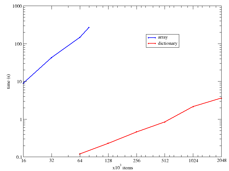
The execution times were so different, and the collection size (nitems) range so wide, I have used a [[logarithmic scale]] for both axes in the time vs collection size below:

At 64k items, the dictionary search is already 3 orders of magnitude faster, and the difference grows fast as the collection size increases.

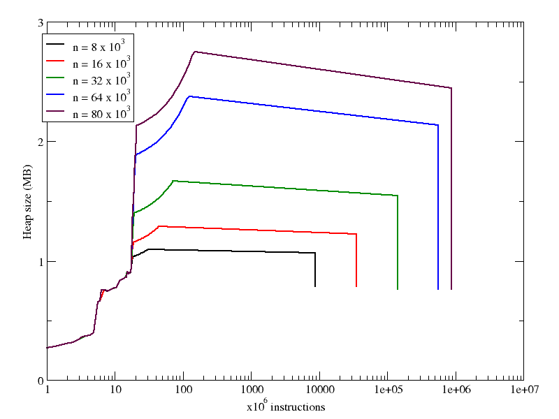
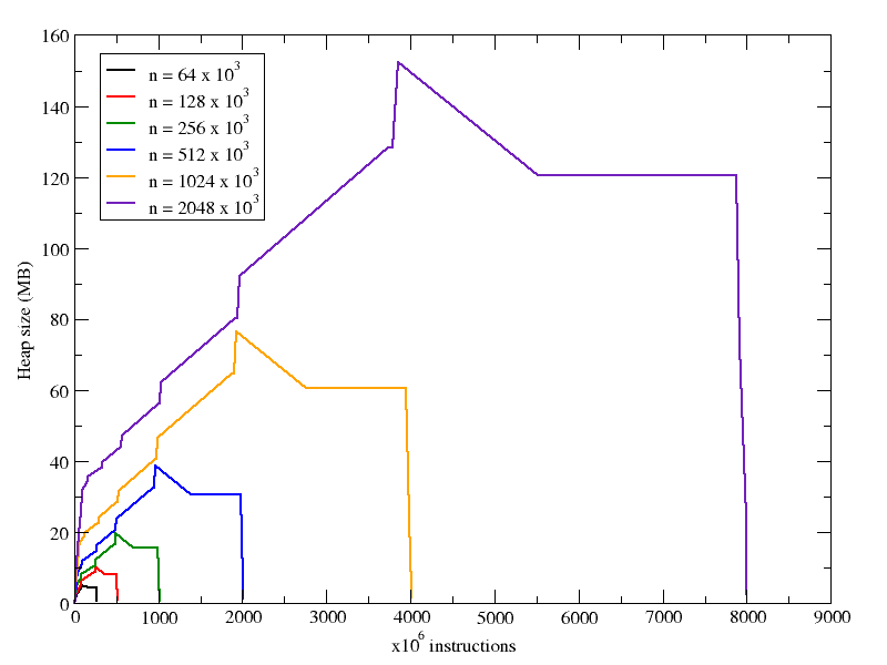
With respect to memory use, we can see that in both cases increasing nitems increases the heap size, but in the case of the arrays, the increase is not so pronounced. Looking at the X axes in both following plots, you can see that the number of instructions executed during the run grows linearly with the number of items in the collection (recall that the array plot has a logarithmic X axis).

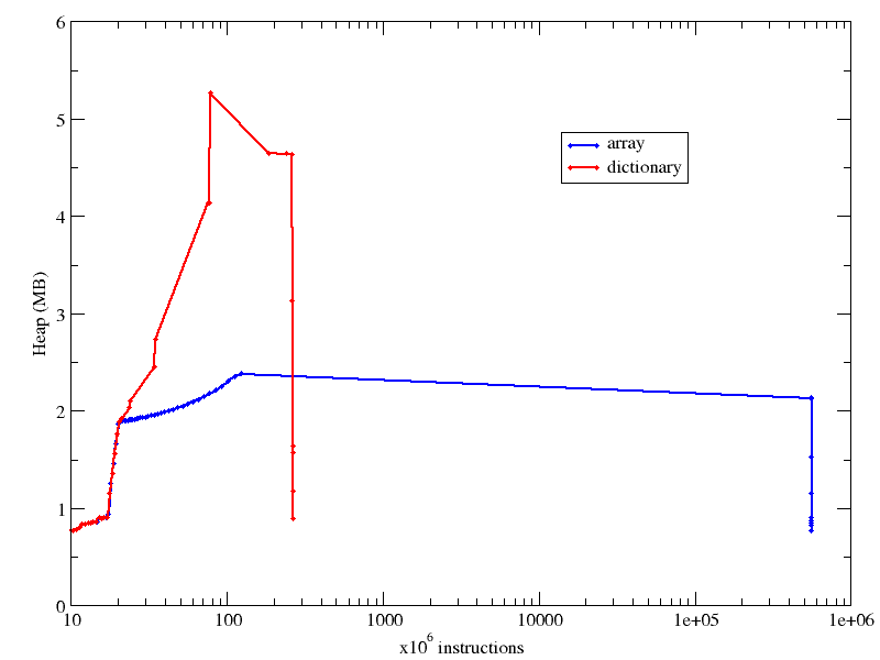
Finally, I compare memory usage of the array and dictionary case in the same plot, as you can see below, for the case of 64k items in the collection:

It wasn’t really an easy task, because I had to combine the biggest array case I could handle with the smallest dictionary the timing of which would be meaningful (smaller dictionaries would be equally “immediate”, according to time). Also notice how the X axis has a log scale. Otherwise the number of instructions in the array case would cross the right border of your monitor.

Update: read second comment

I recently upgraded to [[Ubuntu]] Jaunty Jackalope, and have experienced a much slower response of my desktop since. The problem seems to be with [[Intel GMA]] chips, as my computer has. The reason for the poor performance is that Canonical Ltd. decided not to include the [[UXA]] acceleration in Jaunty, for stability reasons (read more at Phoronix).

The issue is discussed at the Ubuntu wiki, along with some solutions. For me, the fix involved just making [[X.Org Server|X.org]] use UXA, by including the following in the xorg.conf file, as they recommend in the wiki:

Section "Device"
        Identifier    "Configured Video Device"
        # ...
        Option        "AccelMethod" "uxa"
EndSection