handyfloss

This is a continuation post for my Linux World Domination project, started in this May 2008 post. You can read the previous post in the series here.

In the following data T2D means “time to domination” (the expected time for Windows/Linux shares to cross, counting from the present date). DT2D means difference (increase/decrease) in T2D, with respect to last report. CLP means “current Linux Percent”, as given by last logged data, and DD means domination day (in YYYY-MM-DD format).

The numbers (again) seem quite discouraging, but the data is what it is. All CLPs but MalariaControl have gone up, with Spinhenge going up by almost a 0.4% in 3 months. The Linux tide seems unstoppable, however its forward speed is not necessarily high.

As promised, today I’m showing the plots for QMC@home, in next issue Rosetta@home.

Number of hosts percent evolution for QMC@home (click to enlarge)

Accumulated credit percent evolution for QMC”home (click to enlarge)

Update: this script has been superseded by ChopZip

Introduction

I discovered the [[Lempel-Ziv-Markov chain algorithm|LZMA]] compression algorithm some time ago, and have been thrilled by its capacity since. It has higher compression ratios than even [[bzip2]], with a faster decompression time. However, although decompressing is fast, compressing is not: LZMA is even slower than bzip2. On the other hand, [[gzip]] remains blazing fast in comparison, while providing a decent level of compression.

More recently I have discovered the interesting pbzip2, which is a parallel implementation of bzip2. With the increasing popularity of multi-core processors (I have a quad-core at home myself), parallelizing the compression tools is a very good idea. pbzip2 performs really well, producing bzip2-compatible files with near-linear scaling with the number of CPUs.

LZMA being such a high performance compressor, I wondered if its speed could be boosted by using it in parallel. Although the [[Lempel-Ziv-Markov chain algorithm|Wikipedia article]] states that the algorithm can be parallelized, I found no such implementation in Ubuntu 9.04, where the utility provided by the lzma package is exclusively serial. Not finding one, I set myself to produce it.

About plzma.py

Any compression can be parallelized as follows:

1. Split the original file into as many pieces as CPU cores available
2. Compress (simultaneously) all the pieces
3. Create a single file by joining all the compressed pieces, and call the result “the compressed file”

In a Linux environment, these three tasks can be carried out easily by split, lzma itself, and tar, respectively. I just made a [[Python (programming language)|Python]] script to automate these tasks, called it plzma.py, and put it in my web site for anyone to download (it’s GPLed). Please notice that plzma.py has been superseded by chopzip, starting with revision 12, whereas latest plzma is revision 6.

I must remark that, while pbzip2 generates bzip2-compatible compressed files, that is not the case with plzma. The products of plzma compression must be decompressed with plzma as well. The actual format of a plzma file is just a TAR file containing as many LZMA-compressed chunks as CPUs used for compression. These chunks, once decompressed individually, can be concatenated (with the cat command) to form the original file.

Benchmarks

What review of compression tools lacks benchmarks? No matter how inaccurate or silly, none of them do. And neither does mine :^)

I used three (single) files as reference:

• molekel.tar – a 108 MB tar file of the (GPL) [[Molekel]] 5.0 source code
• usr.bin.tar – 309 MB tar file of the contens of my /usr/bin/ dir
• hackable.tar – a 782 MB tar file of the hackable:1 [[Debian]]-based distro for the [[Neo FreeRunner]]

The second case is intended as an example of binary file compression, whereas the other two are more of a “real-life” example. I didn’t test text-only files… I might in the future, but don’t expect the conclusions to change much. The testbed was my Frink desktop PC (Intel Q8200 quad-core).

The options for each tool were:

• gzip/bzip/pbzip2: compression level 6
• lzma/plzma: compression level 3
• pbzip2/plzma: 4 CPUs

Compressed size

The most important feature of a compressor is the size of the resulting file. After all, we used it in first place to save space. No matter how fast an algorithm is, if the resulting file is bigger than the original file I wouldn’t use it. Would you?

The graph below shows the compressed size ratio for compression of the three test files with each of the five tools considered. The compressed size ratio is defined as the compressed size divided by the original size for each file.

This test doesn’t surprise much: gzip is the least effective and LZMA the most one. The point to make here is that the parallel implementations perform as well or badly as their serial counterparts.

If you are unimpressed by the supposedly higher performance of bzip2 and LZMA over gzip, when in the picture all final sizes do not look very different, recall that gzip compressed molekel.tar ~ 3 times (to a 0.329 ratio), whereas LZMA compressed it ~ 4.3 times (to a 0.233 ratio). You could stuff 13 LZMAed files where only 9 gzipped ones fit (and just 3 uncompressed ones).

Compression time

However important the compressed size is, compression time is also an important subject. Actually, that’s the very issue I try to address parallelizing LZMA: to make it faster while keeping its high compression ratio.

The graph below shows the normalized times for compression of the three test files with each of the five tools considered. The normalized time is taken as the total time divided by the time it took gzip to finish (an arbitrary scale with t(gzip)=1.0).

Roughly speaking, we could say that in my setting pbzip2 makes bzip2 as fast as gzip, and plzma makes LZMA as fast as serial bzip2.

The speedups for bzip2/pbzip2 and LZMA/plzma are given in the following table:

The performance of plzma is nowere near pbzip2, but I’d call it acceptable (wouldn’t I?, I’m the author!). There are two reasons I can think of to explain lower-than-linear scalability. The first one is the overhead imposed when cutting the file into pieces then assembling them back. The second one, maybe more important, is the disk performance. Maybe each core can compress each file independently, but the disk I/O for reading the chunks and writing them back compressed is done simultaneously on the same disk, which the four processes share.

Update: I think that a good deal of under-linearity comes from the fact that files of equal size will not be compressed in an equal time. Each chunk compression will take a slightly different time to complete, because some will be easier than others to compress. The program waits for the last compression to finish, so it’s as slow as the slowest one. It is also true that pieces of 1/N size might take more than 1/N time to complete, so the more chunks, the slower the compression in total (the opposite could also be true, though).

Decompression times

Usually we pay less attention to it, because it is much faster (and because we often compress things never to open them again, in which case we had better deleted them in first place… but I digress).

The following graph shows the decompression data equivalent to the compression times graph above.

The most noteworthy point is that pbzip2 decompresses pbzip2-compressed files faster than bzip2 does with bzip2-compressed files. That is, both compression and decompression benefit from the parallelization. However, for plzma that is not the case: decompression is slower than with the serial LZMA. This is due to two effects: first, the decompression part is still not parallelized in my script (it will soon be). This would lead to decompression speeds near to the serial LZMA. However, it is slower due to the second effect: the overhead caused by splitting and then joining.

Another result worth noting is that, although LZMA is much slower than even bzip2 to compress, the decompression is actually faster. This is not random. LZMA was designed with fast uncompression time in mind, so that it could be used in, e.g. software distribution, where a single person compresses the original data (however painstakingly), then the users can download the result (the smaller, the faster), and uncompress it to use it.

Conclusions

While there is room for improvement, plzma seems like a viable option to speed up general compression tasks where a high compression ratio (LZMA level) is desired.

I would like to stress the point that plzma files are not uncompressable with just LZMA. If you don’t use plzma to decompress, you can follow the these steps:

Accessing both Windows [[File Allocation Table|FAT]] and [[NTFS]] file systems from Linux is quite easy, with tools like [[NTFS-3G]]. However (following with the [[shit|MS]] tradition of making itself incompatible with everything else, to thwart competition), doing the opposite (accessing Linux file systems from Windows) is more complicated. One would have to guess why (and how!) [[closed source software|closed]] and [[proprietary software|proprietary]] and technically inferior file systems can be read by free software tools, whereas proprietary software with such a big corporation behind is incapable (or unwilling) to interact with superior and [[free software]] file systems. Why should Windows users be deprived of the choice over [[JFS (file system)|JFS]], [[XFS]] or [[ReiserFS]], when they are free? MS techs are too dumb to implement them? Or too evil to give their users the choice? Or, maybe, too scared that if choice is possible, their users will dump NTFS? Neither explanation makes one feel much love for MS, does it?

This stupid inability of Windows to read any of the many formats Linux can use gives rise to problems for not only Windows users, but also Linux users. For example, when I format my external hard disks or pendrives, I end up wondering if I should reserve some space for a FAT partition, so I could put there data to share with hypothetical Windows users I could lend the disk to. And, seriously, I abhor wasting my hardware with such lousy file systems, when I could use Linux ones.

Anyway, there are some third-party tools to help us which such a task. I found at least two:

• Ext2IFS
• ext2fsd

I have used the first one, but as some blogs point out (e.g. BloggUccio), ext2fsd is required if the [[inode]] size is bigger than 128 B (256 B in some modern Linux distros).

Getting Ext2IFS

It is a simple exe file you can download from fs-driver.org. Installing it consists on the typical windows next-next-finish click-dance. In principle the defaults are OK. It will ask you about activating “read-only” (which I declined. It’s less safe, but I would like to be able to write too), and something about large file support (which I accepted, because it’s only an issue with Linux kernels older than 2.2… Middle Age stuff).

Formatting the hard drive

In principle, Ext2IFS can read ext2/ext3 partitions with no problem. In practice, if the partition was created with an [[inode]] size of more than 128 bytes, Ext2IFS won’t read it. To create a “compatible” partition, you can mkfs it with the -I flag, as follows:

I found out about the 128 B inode thing from this forum thread [es].

Practical use

What I have done, and tested, is what follows: I format my external drives with almost all of it as ext3, as described, leaving a couple of gigabytes (you could cut down to a couple of megabytes if you really want to) for a FAT partition. Then copy the Ext2IFS_1_11a.exe executable to that partition.

Whenever you want to use that drive, Linux will see two partitions (the ext3 and the FAT one), the second one of which you can ignore. From Windows, you will see only a 2GB FAT partition. However, you will be able to open it, find the exe, double-click, and install Ext2IFS. After that, you can unplug the drive and plug it again…et voilà, you will see the ext3 partition just fine.

I started installing [[Ubuntu Netbook Remix]] 9.04 in my [[ASUS Eee PC]], and after the partitioning step, I stumbled upon the following error:

The installer needs to remove operating system files from the install target, but was unable to do so. The install cannot continue

I was installing Ubuntu on top of a previous eeebuntu install, smashing the / partition, while reusing the /home. After minimal googling, I found this bug report at Launchpad, with the same problem (and one year old).

As it turns out, the problem was not with the root partition, as I assumed from the error message, but with the home one. Apparently, Ubuntu didn’t like the idea that my home partition was [[JFS (file system)|JFS]] (maybe it couldn’t mount it, because jfs_utils are not loaded by default). The solution: install the OS ignoring (not using) the home partition, and mount it afterwards.

Shame on you, Ubuntu, this solution is lame!

It’s old news, but I just read about in in the Wikipedia article for the [[Phenom II]] processor.

Apparently Phenom processors had the ability to scale the CPU frequency independently for each core in multicore systems. Now, Phenom II processors lack this feature: the CPU frequency can be scaled, but all cores must share the same frequency.

Did this happen because of technical reasons? AMD thought it was better to do it? No. As Wikipedia says:

Another change from the original Phenom is that Cool ‘n Quiet is now applied to the processor as a whole, rather than on a per-core basis. This was done in order to address the mishandling of threads by Windows Vista, which can cause single-threaded applications to run on a core that is idling at half-speed.

The situation is explained in an article in anandtech.com, where the author mistakes an error on Vista’s account with an error in the Phenom processor (bolding of text is mine):

In theory, the AMD design made sense. If you were running a single threaded application, the core that your thread was active on would run at full speed, while the remaining three cores would run at a much lower speed. AMD included this functionality under the Cool ‘n’ Quiet umbrella. In practice however, Phenom’s Cool ‘n’ Quiet was quite flawed. Vista has a nasty habit of bouncing threads around from one core to the next, which could result in the following phenomenon (no pun intended): when running a single-threaded application, the thread would run on a single core which would tell Vista that it needed to run at full speed. Vista would then move the thread to the next core, which was running at half-speed; now the thread is running on a core that’s half the speed as the original core it started out on.

Phenom II fixes this by not allowing individual cores to run at clock speeds independently of one another; if one core must run at 3.0GHz, then all four cores will run at 3.0GHz. In practice this is a much better option as you don’t run into the situations where Phenom performance is about half what it should be thanks to your applications running on cores that are operating at half speed. In the past you couldn’t leave CnQ enabled on a Phenom system and watch an HD movie, but this is no longer true with Phenom II.

Recall how the brilliant author ascribes the “flaw” to CnQ, instead of to Vista, and how it was AMD who “fixed” the problem!

The plain truth is that AMD developed a technology (independent core scaling) that would save energy (which means money and ecology) with zero-effects on performance (since the cores actually running jobs run at full speed), and MS Vista being a pile of crap forced them to revert it.

Now, if you have a computer with 4 or 8 cores, and watch a HD movie (which needs a full-speed core to decode it, but only one core), the full 8 cores will be running at full speed, wasting power, producing CO₂, and making you get charged money at a rate 8 times that actually required!

The obvious right solution would be to fix Vista so that threads don’t dance from core to core unnecessarily, so that AMD’s CnQ technology could be used to full extent. AMD’s movement with Phenom II just fixed the performance problem, by basically destroying the whole point of CnQ.

Now take a second to reflex how the monstrous domination of MS over the OS market leads to problems like this one. In a really competitive market, if a stupid OS provider gets it wrong and their OS does not support something like CnQ properly, the customers will migrate to other OSs, and the rogue provider will be forced to fix their OS. The dominance of MS (plus their stupidity), just held back precious technological advances!

That’s where you can lodge your [[HADOPI law]], you totalitarian dwarf.

Apparently there is some common sense in the French tribunals, and that stupid law was revoked. Well, not really revoked, just cut down in its most dangerous bit (the ability of the ISPs to shut down the connection of a user based on perceived “pirate” activity). I just read about at Enrique Dans’s blog [es].

I am using the [[Glade Interface Designer]] to produce (very) small (and simple) graphical apps for my [[Neo FreeRunner]]. I produce the graphical layout in the form of an [[XML]] file (using Glade), then load this XML from a [[PyGTK]] program.

The thing is some defaults are not really usable for a device such as the NFR. For example, default fonts are in general too small for the tiny screen of the Neo, which favors apps with only a few, big and shinny buttons. In the case of Label widgets, you can use Pango markup format with the set_markup method, as follows:

mylabel  = self.glade.get_widget('label1')
txt  = '<span font_size="80000" color="red">%s</span>' % (text_string)
mylabel.set_markup(txt)

However, for other widgets it is not so evident. For example, in ComboBoxes (buttons with a drop-down list), you can’t put in the item list anything other than strings, which are displayed literally (markup is not interpreted). Moreover, CBs do not have a “set_font_style” method, or anything similar.

Searching the web did not provide immediate results, but I managed to find this FAQ item at eccentric.cx. I quote:

4.1.581 How do I change font properties on gtk.Labels and other widgets?
Easy:

 label = gtk.Label("MyLabel")
 label.modify_font(pango.FontDescription("sans 48"))

This method applies to all widgets that use text, so you can change the text of gtk.Entry and other widgets in the same manner.

Note that, some widgets are only containers for others, like gtk.Button. For those you’d have to get the child widget. For a gtk.Button do this:

  if button.get_use_stock():
     label = button.child.get_children()[1]
  elif isinstance(button.child, gtk.Label):
     label = button.child
  else:
     raise ValueError("button does not have a label")

Last changed on Thu Sep 1 14:46:30 2005 by Johan Dahlin (johan-at-gnome-org)

In the case of a CB, we have to pick its child (which is the list itself), and modify it thusly:

cbox = self.glade.get_widget("CBlist")
cblist  = cbox.child
cblist.modify_font(pango.FontDescription("sans 32"))

In my examples above, a class has been created in the script beforehand, and it binds to the Glade XML:

class whatever:

  def __init__(self):

    #Set the Glade file
    self.glade    = gtk.glade.XML(gladefile)
    self.glade.signal_autoconnect(self)

Of course, the CBlist and MyLabel mentioned in my code are the appropriate widget names defined in that XML.

As you can see in this war-time poster by the USA government, the official policy on oil (ab)use has not always been “waste as much as you can”:

I found the picture in the [[carpool]] Wikipedia article.

This is a continuation post for my Linux World Domination project, started in this May 2008 post. You can read the previous post in the series here.

In the following data T2D means “time to domination” (the expected time for Windows/Linux shares to cross, counting from the present date). DT2D means difference (increase/decrease) in T2D, with respect to last report. CLP means “current Linux Percent”, as given by last logged data, and DD means domination day (in YYYY-MM-DD format).

For the first time, data for [[PrimeGrid]] is included.

Mmm, the numbers seem quite discouraging, but the data is what it is. On the bright side, all CLPs have gone up, some almost a 0.3% in 3 months. The Linux tide seems unstoppable, however its forward speed is not necessarily high.

As promised, today I’m showing the plots for PrimeGrid, in next issue QMC@home.

Number of hosts percent evolution for PrimeGrid (click to enlarge)

Accumulated credit percent evolution for PrimeGrid (click to enlarge)

I guess this post is not going to reveal anything new: testing for an item’s membership in an array is slow, and dictionaries are much more CPU-efficient for that (albeit more RAM-hungry). I’m just restating the obvious here, plus showing some benchmarks.

Intro

Let’s define our problem first. We simply want to check whether some item (a string, number or whatever) is contained within some collection of items. For that, the simplest construct in [[Python (programming language)|Python]] would be:

if item in collection:
  do something

The above construct works regardless of “collection” being an array or a dictionary. However, the search for “item” in “collection” is different internally. In the case of a list, Python checks all its elements one by one, comparing them to “item”. If a match is found, True is returned, and the search aborted. For items not in the list, or appearing very late inside it, this search will take long.

However, in the case of dictionaries, the search is almost a one-step procedure: if collection[item] returns something other than an error, then item is in collection.

The tests

I’ve run two different test scripts, one for the array case, another for the dictionary case. In both cases I’ve searched for an item that was not in the collection, to maximize the searching efforts. The array script was as follows:

#!/usr/bin/python

import sys

nitems = int(sys.argv[1])

foo = []
bar = []

for i in range(nitems):
 foo.append(1)
 bar.append(2)

for i in foo:
  if i in bar:
    pass

Similarly, for dictionaries:

#!/usr/bin/python

import sys

nitems = int(sys.argv[1])

foo = {}
bar = {}

for i in range(nitems):
  j = i + nitems
  foo[i] = True
  bar[j] = True

for i in foo:
  if i in bar:
    pass

Both scripts accept (require) an integer number as argument, then build item collections of this size (initialization), then run the check loops. The loops are designed to look for every item of collection 1 in collection 2 (and all checks will fail, because no single item belongs to both sets).

Timing

The scripts were timed simply by measuring the execution [[wall clock time|walltime]] with the GNU time command, as follows:

Bear in mind that the computer was not otherwise idle during the tests. I was surfing the web with Firefox and listening to music with Amarok. Both programs are CPU- and (specially) memory-hungry, so take my results with a grain of salt. In any case, it was not my intention to get solid numbers, but just solid trends.

Memory profiling

I must confess my lack of knowledge around memory management of software, and how to profile it. I just used the [[Valgrind]] utility, with the massif tool, as follows:

% valgrind --tool=massif script nitems

Massif creates a log file (massif.out.pid) that contains “snapshots” of the process at different moments, and gives each of them a timestamp (the default timestamp being the number of instructions executed so far). The logged info that interests us is the [[dynamic memory allocation|heap]] size of the process. As far as I know (in my limited knowledge), this value corresponds to the RAM memory allotted to the process. This value can be digested out of the log file into a format suitable for printing heap size vs. execution time (instructions, really), by a Python script:

#!/usr/bin/python

import sys

try:
  fn = sys.argv[1]
except:
  sys.exit('Insert file name')

b2m = 1024*1024
e2m = 1000000

f = open(fn,'r')

for line in f:
  if 'time=' in line:
    aline = line.split('=')
    t     = aline[1].replace('\n','')
    t     = float(t)/e2m

  elif 'mem_heap_B' in line:
    aline = line.split('=')
    m     = aline[1].replace('\n','')
    m     = float(m)/b2m

    print t,m

f.close()

The above outputs heap MB vs million executions.

A much conciser form with [[AWK|awk]]:

% awk -F= '/time=/{t=$2/1000000};/mem_heap_B/{print t, $2/1048576}' massif.out.pid

Results

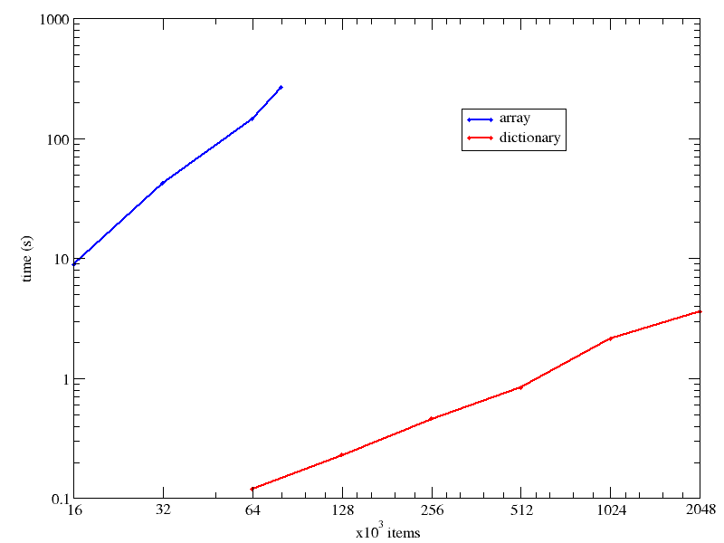
The execution times were so different, and the collection size (nitems) range so wide, I have used a [[logarithmic scale]] for both axes in the time vs collection size below:

At 64k items, the dictionary search is already 3 orders of magnitude faster, and the difference grows fast as the collection size increases.

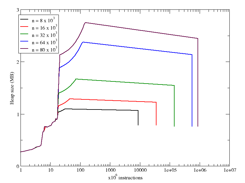
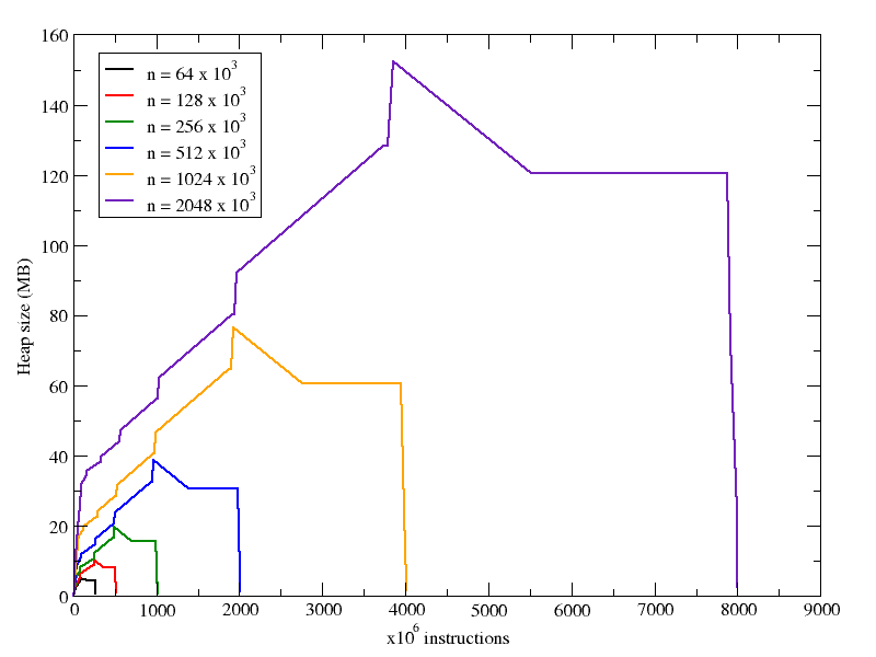
With respect to memory use, we can see that in both cases increasing nitems increases the heap size, but in the case of the arrays, the increase is not so pronounced. Looking at the X axes in both following plots, you can see that the number of instructions executed during the run grows linearly with the number of items in the collection (recall that the array plot has a logarithmic X axis).

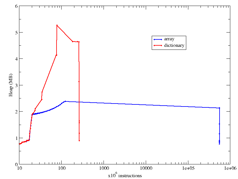
Finally, I compare memory usage of the array and dictionary case in the same plot, as you can see below, for the case of 64k items in the collection:

It wasn’t really an easy task, because I had to combine the biggest array case I could handle with the smallest dictionary the timing of which would be meaningful (smaller dictionaries would be equally “immediate”, according to time). Also notice how the X axis has a log scale. Otherwise the number of instructions in the array case would cross the right border of your monitor.